Grothendieck residues on zero-dimensional complete intersections
As part of an ongoing project with Ran Azouri and Felipe Espreafico Guelerman, I have recently discovered that the Scheja–Storch residue [SS75] (used to define the Eisenbud–Khimshiashvili–Levine form, and hence the quadratic (aka \(\mathbb{A}^1\)-)Milnor number) is actually an incarnation of the more general concept of Grothendieck residues. What follows is my best attempt to explain, mostly to myself, what these residues are in terms of abstract nonsense that I already understand. I learnt this from [Dég23, § 6.3], so you can just read that if you want a different exposition of the same story. At the end of the post I have included an explanation of the relationship with the classical residue of a meromorphic differential form on a Riemann surface.
Grothendieck duality and dualizing complexes
The starting point of our discussion is Grothendieck duality, also known as coherent duality. It is the analog of Verdier duality in the context of schemes and coherent sheaves.
Super-duper general duality results
The latest versions of Grothendieck duality divide the result into two parts.
Theorem 1 (existence of a right adjoint, [Nee23, § 2]) Let \(f: X \to Y\) be a qcqs morphism of schemes (also works for concentrated morphisms of algebraic stacks). Then the derived pushforward functor \(\mathbf{R}f_*: \mathsf{D_{qc}}(X) \to \mathsf{D_{qc}}(Y)\) admits a right adjoint \(f^\times: \mathsf{D_{qc}}(Y) \to \mathsf{D_{qc}}(X)\).
Theorem 2 (properties of the exceptional pullback, [Nee23, Thm. 1.8, 1.8.1-1.8.10, Rem. 1.13, Rem. 1.14]) There is a contravariant oplax functor \((-)^!\) from the category of noetherian schemes with separated morphisms essentially of finite type to the category of triangulated categories, sending \(X \mapsto \mathsf{D_{qc}}(X)\) and \((f: X \to Y) \mapsto (f^!: \mathsf{D_{qc}}(Y) \to \mathsf{D_{qc}}(X))\). It has the following properties:
There is a natural transformation \((-)^\times \to (-)^!\) which is an isomorphism when \(f\) is proper.
The natural map \((g \circ f)^! \to f^! \circ g^!\) is an isomorphism if \(f\) has finite Tor-dimension, or if \(g\) or \(g \circ f\) is proper, or after restricting to \(\mathsf{D}^+_{qc}\).
It satisfies flat base change, i.e. there is a natural map \(\theta:\;L(g')^*f^! \to (f')^!Lg^*\) which is an isomorphism when \(g\) is flat (+ some finiteness condition on \(f'\) if we want unbounded complexes).
If \(j\) is an open immersion, then \(j^! \cong j^*\). Thus if \(f = pj\) with \(j\) open and \(p\) proper, then \(f^! \cong j^*p^\times\).
For our purposes, we will only need Grothendieck duality for morphisms of affine schemes, in which case the proof is elementary.
Corollary 3 Let \(A, B\) be noetherian rings, and let \(f: \Spec B \to \Spec A\) be a finite morphism (recall that affine + proper = finite [Stacks], Tag 01WN). Then \(\mathbf{R}f_*: \mathsf{D}(B) \to \mathsf{D}(A)\), which is just restriction of scalars, admits a right adjoint \(f^!\), which is given by coextension of scalars \[ f^!(-) = \mathbf{R}\Hom_A(B, -). \] The counit \(\mathbf{R}f_*f^! \to \id\) is called the trace map, denoted \(\tr_{B/A}\), and it is given by evaluation at \(1 \in B\).
Remark. Corollary 3 is just a fancy rewording of the tensor-Hom adjunction. The result holds for general finite morphisms of schemes, and the proof is still elementary, see [Stacks], Tag 0AWZ.
The reason why we care about Grothendieck duality, and why we have placed Corollary 3 in this context, is that it allows us to define a dualizing complex for any separated \(k\)-scheme of finite type \(a: X \to \Spec k\), namely \(\omega_X^\bullet \coloneqq a^!k\). This is dualizing in the usual categorical sense [Dég23, Def. 6.1.11], i.e. it defines a functor \(\mathbf{D}_X \coloneqq \mathbf{R}\sHom_X(-, \omega_X^\bullet): \mathsf{D^b_{coh}}(X) \to \mathsf{D^b_{coh}}(X)^\mathrm{op}\) such that the natural transformation \(\id \to \mathbf{D}_X \circ \mathbf{D}_X\) is an isomorphism.
The dualizing complex becomes less abstract when we impose some additional hypotheses on \(X\). Indeed, if \(X\) is equidimensional of dimension \(n\), then:
- \(\omega_X^\bullet\) is a shifted sheaf if and only if \(X\) is Cohen–Macaulay (more precisely, \(\omega_X^\bullet \cong \mathcal{F}[n]\) for a coherent sheaf \(\mathcal{F}\), [Stacks], Tag 0AWQ).
- \(\omega_X^\bullet\) is a shifted line bundle if and only if \(X\) is Gorenstein (more precisely, \(\omega_X^\bullet \cong \mathcal{L}[n]\) for a line bundle \(\mathcal{L}\), [Stacks], Tag 0AWV).
- If \(X\) is smooth over \(k\), then \(\omega_X^\bullet \cong \bigwedge^n\Omega^1_{X/k}[n]\). If one uses the typical notation \(\omega_X \coloneqq \bigwedge^n\Omega^1_{X/k}\), this becomes the potentially confusing formula \(\omega_X^\bullet \cong \omega_X[n]\).
The dualizing sheaf of a zero-dimensional complete intersection
Let \(i: P \hookrightarrow X\) be a closed immersion of \(k\)-schemes, with \(X/k\) smooth of dimension \(n\), and \(P\) a zero-dimensional complete intersection. Working locally at a point of \(P\), we may restrict to an affine open neighborhood and assume that \(X = \Spec R\) and \(P = \Spec R/(\mathbf t)\), where \(\mathbf t = (t_1, \ldots, t_n)\) is a regular sequence.
Put \(X = \mathbb{A}^n_k\) and let \(f \in k[x_1, \ldots, x_n]\) have an isolated critical point at the (rational) origin, i.e. \(0\) is an isolated point of \(V(\partial_1 f, \ldots, \partial_n f)\). The local ring \(k[x]_{(x)}\) is Cohen–Macaulay of dimension \(n\), each \(\partial_i f\) lies in its maximal ideal, and the quotient by \((\partial_1 f, \ldots, \partial_n f)\) has dimension \(0 = n - n\), so \(\mathbf t = (\partial_1 f, \ldots, \partial_n f)\) is a regular sequence in this local ring by [Stacks], Tag 02JN, hence on a neighborhood of \(0\). After restricting to a sufficiently small affine open neighborhood of \(0\), the critical locus \(P\) is therefore defined by the regular sequence \(\mathbf t\), and its coordinate ring is the local Milnor algebra \(k[x]_{(x)}/J(f)\).
Observe that both \(X\) and \(P\) are Cohen–Macaulay, so their dualizing complexes are sheaves, and we write \(\omega_X^\bullet \cong \omega_X[n]\) and \(\omega_P^\bullet \cong \omega_P[0]\). As usual, we will identify sheaves of \(\mathcal{O}_X\)-modules with their \(R\)-module of global sections.
Lemma 4 There is an isomorphism of \(R/(\mathbf t)\)-modules \[ \omega_P \cong i^* \omega_X \otimes \det((\mathbf t)/(\mathbf t)^2)^\vee. \] Therefore, fixing a generator \(\sigma\) of \(\omega_X\) gives a generator \(\xi_{\sigma, \mathbf t}\) of \(\omega_P\), namely the one corresponding to \(\sigma|_P \otimes (\bar{t}_1 \wedge \cdots \wedge \bar{t}_n)^\vee\) under the isomorphism above.
Proof. Writing \(a_X\) and \(a_P\) for the structure morphisms, we have \(a_P = a_X \circ i\). Here \(a_P\) is finite, hence proper, so by part (2) of Theorem 2 we get \(\omega_P^\bullet = (a_X \circ i)^! k \cong i^! a_X^! k = i^! \omega_X^\bullet\). Since \(i\) is finite, we can apply Corollary 3 and obtain \[ i_*\omega_P % \cong i_* i^! \omega_X[n] % \cong i_* \mathbf{R}\Hom_{R/(\mathbf t)} \bigl(R/(\mathbf t), i^! \omega_X[n]\bigr) \cong \mathbf{R}\Hom_R \bigl(R/(\mathbf t), \omega_X[n]\bigr). \] Here we write \(i_*\) rather than \(\mathbf{R}i_*\) because \(i\) is a closed immersion, hence affine, so \(i_*\) is exact and needs no deriving; concretely, it is just restriction of scalars along \(R \to R/(\mathbf t)\).
Recall that regularity of the sequence \(\mathbf t\) implies that the Koszul complex \[ K(\mathbf t): \bigwedge^n F \to \cdots \to F \to R \] is a free resolution of \(R/(\mathbf t)\), where \(F = R^{\oplus n}\) and the differentials are given by contraction with \(\mathbf t\) (we are using cohomological grading, i.e. \(K(\mathbf t)^k = \bigwedge^{-k} F\)). Using this resolution, we can compute the derived Hom above. Since \(i_*\omega_P\) is concentrated in degree \(0\) so is the \(\mathbf{R}\Hom\), hence its only nontrivial cohomology is the cokernel of the map \[ \Hom_R(\bigwedge^{n-1} F, \omega_X) \xlongrightarrow{(d^{-n}_{K(\mathbf t)})^*} \Hom_R(\bigwedge^n F, \omega_X). \tag{1}\] Evaluating on the bases \(e_1 \wedge \cdots \wedge e_n\) of \(\bigwedge^n F\) and \(\{e_1 \wedge \cdots \wedge \widehat{e_i} \wedge \cdots \wedge e_n\}_{i = 1, \ldots, n}\) of \(\bigwedge^{n-1} F\) identifies (1) with \(\omega_X^{\oplus n} \to \omega_X: (\alpha_1, \ldots, \alpha_n) \mapsto \sum_{i=1}^n (-1)^{i+1} t_i \alpha_i\), whose image is \((\mathbf t)\omega_X\). Now we just compute \[ \begin{aligned} \omega_P &\cong i^* i_*\omega_P \cong i^*\bigl( \Hom_R(\textstyle\bigwedge^n F, \omega_X) / (\mathbf t) \bigr) \\[-0.4ex] &\qquad\text{\small by the computations above,} \\ &\cong \left( \Hom_R(\textstyle\bigwedge^n F, \omega_X) \otimes_R R/(\mathbf t) \right) \otimes_R R/(\mathbf t) \\[-0.4ex] &\qquad\text{\small since $i^*$ is extension of scalars,} \\ &\cong \Hom_R(\textstyle\bigwedge^n F, \omega_X) \otimes_R R/(\mathbf t) \\[-0.4ex] &\qquad\text{\small as this is already an $R/(\mathbf t)$-module,} \\ &\cong \Hom_{R/(\mathbf t)}\left( \textstyle\bigwedge^n F \otimes_R R/(\mathbf t), \omega_X \otimes_R R/(\mathbf t) \right) \\[-0.4ex] &\qquad\text{\small since $\textstyle\bigwedge^n F$ is finite free,} \\ &\cong \Hom_{R/(\mathbf t)}\left( \textstyle\bigwedge^n (F \otimes_R R/(\mathbf t)), i^*\omega_X \right) \\[-0.4ex] &\qquad\text{\small because exterior powers commute with extension of scalars,} \\ &\cong \Hom_{R/(\mathbf t)}\left( \textstyle\bigwedge^n ((\mathbf t) \otimes_R R/(\mathbf t)), i^*\omega_X \right) \\[-0.4ex] &\qquad\text{\small by regularity of the sequence $\mathbf t$,} \\ &\cong i^*\omega_X \otimes_{R/(\mathbf t)} \det((\mathbf t)/(\mathbf t)^2)^\vee \\[-0.4ex] &\qquad\text{\small by duality for finite free modules.} \end{aligned} \] This finishes the proof of the isomorphism. Tracing the isomorphisms, \(\sigma|_P \otimes (\bar t_1 \wedge \cdots \wedge \bar t_n)^\vee\) corresponds to the class of the functional \(e_1 \wedge \cdots \wedge e_n \mapsto \sigma\) (here \(F \otimes_R R/(\mathbf t) \cong (\mathbf t)/(\mathbf t)^2\) sends \(e_i \mapsto \bar t_i\)). This is exactly the generator \(\xi_{\sigma, \mathbf t}\).
Definition of the Grothendieck residue
Let \(i: Z \hookrightarrow X\) be a closed immersion of \(k\)-schemes, with ideal sheaf \(\mathcal{I}\). Applying \(\mathbf{R}\sHom_X(-, \omega_X^\bullet)\) to the defining short exact sequence of \(\mathcal{I}\) gives a distinguished triangle \[ \mathbf{R}\sHom_X(i_*\mathcal{O}_Z, \omega_X^\bullet) \rightarrow \mathbf{R}\sHom_X(\mathcal{O}_X, \omega_X^\bullet) \rightarrow \mathbf{R}\sHom_X(\mathcal{I}, \omega_X^\bullet) \xrightarrow{+1}. \tag{2}\]
Definition 5 The residue map associated to \(i: Z \hookrightarrow X\) is the map \[ \rho_{Z/X}: \mathbf{R}\sHom_X(\mathcal{I}, \omega_X^\bullet) \longrightarrow i_* \omega_Z^\bullet[1] \] obtained as the composition of the connecting morphism in the triangle (2) with the Grothendieck duality isomorphism.
As before, this becomes less abstract in particular situations. For example, if \(X\) is smooth of dimension \(n\) and \(Z = D\) is a Cartier divisor, then \(\mathcal{I} = \mathcal{O}_X(-D)\) and \(\rho_{Z/X}[-n]\) is the quotient map in the adjunction sequence \[ 0 \longrightarrow \omega_X \longrightarrow \omega_X(D) \longrightarrow i_* \omega_D \longrightarrow 0, \] i.e. the residue map realizes the adjunction isomorphism \(\omega_X(D)|_D \cong \omega_D\).
We are interested in the case where \(X\) is smooth of dimension \(n\) and \(Z = P\) is a zero-dimensional complete intersection defined by a regular sequence \(\mathbf t = (t_1, \ldots, t_n)\). Observe that \(P\) being zero-dimensional means that \(R/(\mathbf t)\) is a finite-dimensional \(k\)-vector space, so the structure morphism \(a_P: P \to \Spec k\) is finite. Therefore, Corollary 3 gives a trace map \[ \tr_{P/k}: \omega_P \longrightarrow \omega_{\Spec k} = k. \]
Definition 6 Shrinking \(X\) if necessary so that \(\omega_X\) is free of rank one, choose a generator \(\sigma\) of \(\omega_X\). For any \(w = u\sigma \in \omega_X\), the Grothendieck residue symbol is defined as \[ \mathrm{Res} \left[ \frac{w}{\mathbf t} \right] \coloneqq \tr_{P/k}(\bar{u} \xi_{\sigma, \mathbf t}) \in k, \] where \(\bar{u}\) denotes the class in \(R/(\mathbf t)\).
This agrees with the definition given in [Har66, § 9] up to a sign depending only on conventions. The sign can be fixed by requiring \(\mathrm{Res}\left[\tfrac{dx_1 \wedge \cdots \wedge dx_n}{x_1, \ldots, x_n}\right] = 1\) on \(X = \mathbb{A}^n_k\) with \(\mathbf t = (x_1, \ldots, x_n)\), after which the two definitions are exactly equal.
The relationship between the residue map and the Grothendieck residue symbol comes from interpreting the formal fraction \(\left[\tfrac{w}{\mathbf t}\right]\) as a class in the cokernel of the last Koszul differential. More precisely, assuming \(n \geq 2\) (the case \(n = 1\) is discussed below), the truncated Koszul complex \(\bigwedge^n F \to \cdots \to F \to (\mathbf t)\) is exact, and thus gives a free resolution of \((\mathbf t)\) that we can use to compute the derived Hom. We hope the following diagram helps clarify this mess of isomorphisms.
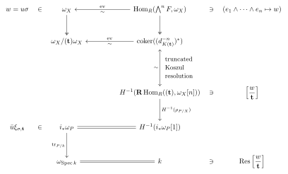
When \(n = 1\), write \(\mathbf t = (t)\), so that \(P\) is a Cartier divisor. The ideal \((t)\) is free of rank one, and hence \[ H^{-1}\mathbf{R}\Hom_R((t), \omega_X[1]) = \Hom_R((t), \omega_X) \cong \omega_X(P). \] Under this identification, the functional sending \(t \mapsto w\) corresponds to the meromorphic differential \(w/t\). The dualizing triangle gives the exact sequence \[ 0 \longrightarrow \omega_X \longrightarrow \omega_X(P) \xlongrightarrow{H^{-1}(\rho_{P/X})} i_*\omega_P \longrightarrow 0. \] Explicitly, for \(w = u\sigma\), the last map sends \[ \frac{w}{t} \longmapsto \bar u\,\xi_{\sigma,t}. \] Thus the Grothendieck residue symbol is again obtained by applying the residue map and then the trace: \[ \mathrm{Res}\left[\frac{w}{t}\right] = \tr_{P/k}\!\left(H^{-1}(\rho_{P/X})(w/t)\right). \] The difference from \(n \geq 2\) is that \(H^{-1}(\rho_{P/X})\) is now a quotient map rather than an isomorphism: its kernel consists of regular differentials.
The key observation is that, while the residue map \(\rho_{P/X}\) is defined abstractly and hence does not depend on any choice, the assignment \(w \mapsto \left[\tfrac{w}{\mathbf t}\right]\) depends on the choice of regular sequence through the Koszul resolution, and the generator \(\xi_{\sigma, \mathbf t} \in \omega_P\) furthermore depends on the choice of a generator \(\sigma \in \omega_X\).
Behavior under morphisms
Let \(Q \hookrightarrow P \hookrightarrow X\) be closed immersions of \(k\)-schemes, with \(X/k\) smooth of dimension \(n\), and \(P, Q\) zero-dimensional complete intersections (in \(X\)). Once again, we may work locally at a point of \(Q\) and assume that \(X = \Spec R\), with \(P\) and \(Q\) being defined by regular sequences \(\mathbf t = (t_1, \ldots, t_n)\) and \(\mathbf s = (s_1, \ldots, s_n)\), respectively.
Since \((\mathbf t) \subset (\mathbf s)\), we can choose a matrix \(A = (a_{ij}) \in R^{n \times n}\) such that \(\mathbf t = A \mathbf s\) (i.e. \(t_i = \sum_j a_{ij} s_j\)). This induces a map of Koszul resolutions
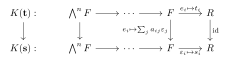
where the left arrow sends \(e_1 \wedge \cdots \wedge e_n \mapsto (\det A) \varepsilon_1 \wedge \cdots \wedge \varepsilon_n\). This represents the quotient map \(R/(\mathbf t) \twoheadrightarrow R/(\mathbf s)\) in the derived category, thus inducing by precomposition a map

This map is just the trace \(\tr_{Q/P}\). Using Grothendieck residue symbols, this becomes the usual residue transformation formula (i.e. Hartshorne’s (R1)): \[ \mathrm{Res} \left[ \frac{w}{\mathbf s} \right] = \mathrm{Res} \left[ \frac{\det(A) \, w}{\mathbf t} \right]. \]
Relationship with the Scheja–Storch residue
Let \(R = k[x_1, \ldots, x_n]\), let \(\mathbf t = (t_1, \ldots, t_n)\) be a regular sequence in \(R\) such that \(B = R/(\mathbf t)\) is finite over \(k\), and let \(\sigma = dx_1 \wedge \cdots \wedge dx_n\). Scheja and Storch [SS75, Satz 3.3] construct a \(k\)-linear map \(\tau_{\mathbf t}: B \to k\) as follows. Choose \(a_{ij} \in R \otimes_k R\) such that \[ t_j \otimes 1 - 1 \otimes t_j = \sum_i a_{ij}\,(x_i \otimes 1 - 1 \otimes x_i) \in R \otimes_k R, \] and let \(\Delta\) be the image of \(\det(a_{ij})\) under the map \(R \otimes_k R \to B \otimes_k B\). The element \(\Delta\) is called the Bezoutian, and is independent of the choice of the \(a_{ij}\) [SS75, Satz 3.1(\(\alpha\))] (but it depends on \(x_1, \ldots, x_n\) and on \(\mathbf t\)). Then \(\tau_{\mathbf t}\) is defined to be the unique \(k\)-linear map \(B \to k\) satisfying \((\tau_{\mathbf t} \otimes \mathrm{id})(\Delta) = 1\) [SS75, Satz 3.3]. According to [Dég23, Prop. 6.3.12], \(\tau_{\mathbf t}\) agrees with the Grothendieck residue: for every \(\lambda \in R\), \[ \mathrm{Res}\left[\frac{\lambda\,dx_1 \wedge \cdots \wedge dx_n}{\mathbf t}\right] = \tau_{\mathbf t}(\bar\lambda). \tag{3}\] We can reword this in our more invariant definition of the residue. Indeed, since \(\omega_P = \Hom_k(B, k)\) and \(\tr_{P/k}\) is evaluation at \(1\), the generator \(\xi_{\sigma, \mathbf t} \in \omega_P\) introduced above is a \(k\)-linear functional on \(B\) and \(\mathrm{Res}\left[\frac{\lambda\,\sigma}{\mathbf t}\right] = \xi_{\sigma, \mathbf t}(\bar\lambda)\). Thus (3) just states \(\xi_{\sigma, \mathbf t} = \tau_{\mathbf t}\).
Let \(\mathrm{Tr}_{B/k}: B \to k\) be the usual trace, sending \(b\) to the trace of the multiplication map \(x \mapsto bx\) on the \(k\)-vector space \(B\). (Warning! This is different from \(\tr_{P/k}\): for instance, it vanishes for any inseparable field extension.) Scheja and Storch show [SS75, Satz 4.2] that \(\mathrm{Tr}_{B/k}(\lambda) = \tau_{\mathbf t}(\bar J \lambda)\), where \(J = \det(\partial t_i/\partial x_j)\) is the Jacobian determinant. Taking \(\lambda = 1\) gives \(\tau_{\mathbf t}(\bar J) = \mathrm{Tr}_{B/k}(1) = \dim_k B\), while (3) applied to \(\lambda = J\) gives \(\tau_{\mathbf t}(\bar J) = \mathrm{Res}[J\,dx_1 \wedge \cdots \wedge dx_n/\mathbf t]\). Therefore \[ \mathrm{Res}\left[\frac{J\,dx_1 \wedge \cdots \wedge dx_n}{\mathbf t}\right] = \dim_k B \in k. \] For \(\mathbf t = (\partial_1 f, \ldots, \partial_n f)\) we have \(J = \det(\partial_i \partial_j f)\), the Hessian determinant, so this says that the residue of the Hessian determinant is the dimension of the Milnor algebra \(k[x_1, \ldots, x_n]/(\partial_1 f, \ldots, \partial_n f)\).
Relationship with classical residues
Let \(k = \mathbb{C}\) and \(n = 1\). Let \(\eta = \sum_{k \geq -m} a_k z^k\,dz\) be the Laurent expansion at \(0\) of a meromorphic form on \(\mathbb{A}^1\). Recall that the classical residue of \(\eta\) at \(0\) is the coefficient \(a_{-1}\), or equivalently the integral \(\frac{1}{2\pi i}\oint_{|z| = \varepsilon} \eta\) over a small circle around \(0\).
Write \(\eta = f\,dz/z^m\) with \(f = \sum_{k \geq 0} a_{k-m} z^k\) holomorphic, and consider the regular sequence \(\mathbf t = (z^m)\), so that \(B = \mathbb{C}[z]/(z^m)\) has basis \(1, z, \ldots, z^{m-1}\). Taking \(t = z^m\), the map described above sends \(f\,dz/z^m\) to \(\bar f\,\xi_{dz,z^m}\). It remains to show that the trace of this element is the coefficient of \(z^{-1}dz\).
Since \(z^m \otimes 1 - 1 \otimes z^m = \bigl(\sum_{i+j=m-1} z^i \otimes z^j\bigr)(z \otimes 1 - 1 \otimes z)\), the Bezoutian is \(\Delta = \sum_{i+j=m-1} z^i \otimes z^j\), and the defining condition of the Scheja–Storch form \((\tau_{\mathbf t} \otimes \mathrm{id})(\Delta) = 1\) reads \(\sum_{i=0}^{m-1} \tau_{\mathbf t}(z^i)\,z^{m-1-i} = 1\) in \(B\). Comparing the coefficients of \(1, z, \ldots, z^{m-1}\) gives \(\tau_{\mathbf t}(z^{m-1}) = 1\) and \(\tau_{\mathbf t}(z^i) = 0\) for \(i < m-1\), i.e. \(\tau_{\mathbf t} = (z^{m-1})^*\) is the coordinate of the last basis vector (cf. [Dég23, Ex. 6.3.9]). Since the right-hand side of (3) only depends on \(f\) modulo \(z^m\), we get \[ \mathrm{Res}\left[\frac{f\,dz}{z^m}\right] = \tau_{\mathbf t}(\bar f) = a_{-1}, \] proving that the Grothendieck residue coincides with the classical residue in this case.